A · Kept model
Closest approach · telescope view
 Contact
Worlds beyond the photograph
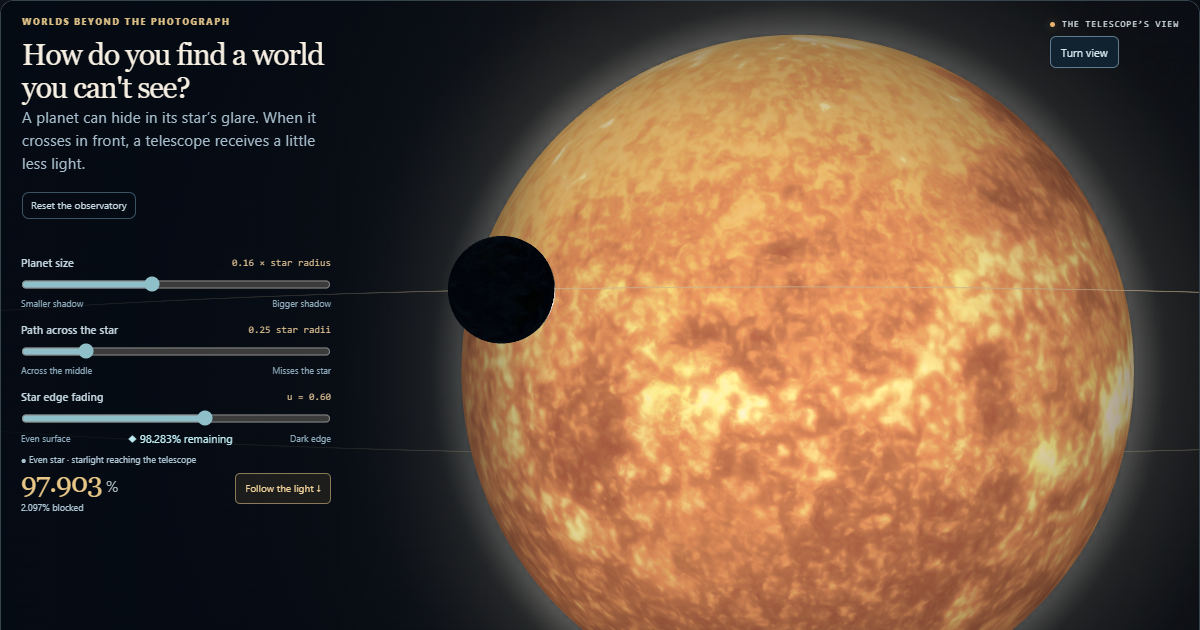
When a planet crosses its star, less starlight reaches the telescope. Drag the planet to see the reading change. In 3D, drag the star or sky to turn your view.
ONE CHANGE. TWO SIGNALS.
Two invented examples · not measurements of a real system
A keeps your original setup; B is yours to change. Start with planet size: a bigger planet can block more starlight and make a deeper dip. Change one setting at a time to see its effect.
Closest approach · telescope view
Closest approach · telescope view
Deeper means more light blocked; wider means a crossing spans more of this model’s orbit. Both plots use the same scales: 155–205° and 85–100% of unblocked light. Pictures show each model’s closest apparent pass to the star; the dots follow your slider.
A bigger silhouette can remove more light. A path nearer the star’s edge can make a shallower, shorter crossing. Fainter star edges change which parts of the crossing remove the most light. Try one change at a time; several changes can partly cancel each other.
Both cards use the adjustable star profile. At u = 0 the surface is evenly bright; at u = 1 its edge fades to zero. Each curve starts at 100% of its own star’s light. The discs are scale diagrams, not measured images.
The same circular orbit and finite-planet brightness calculation drive the main instrument and these plots. A lap has no fitted duration in hours. These are invented models, not fits to WASP-126. The 993 real readings in room 03 are unchanged. Looking around only moves your viewpoint; the telescope stays fixed.
Keep this setup also saves A and whether this comparison is open. Back to the orbit keeps A; End comparison and Reset clear it.
Drag either graph. The shadow beside it shows how much of the star is covered at that moment.
AN EXAMPLE CROSSING · YOUR ORBIT SETTINGS ARE SAVED
The shadow and both markers show the same moment.
2.097% blocked + 97.903% remains
Only part of the planet covers the star here: 2.097% is blocked and 97.903% reaches the telescope. The gold dot marks the light that still arrives.
Circle and diamond show this moment. The pale band marks the close-up; both graphs keep the same brightness scale. ● Gold: even star · ◆ Dashed: dimmer edges
Drag either light curve to move the same planet. Left and right arrows move one degree, Shift moves five degrees, Home goes to zero and End goes to 360.
The close-up shows 155 to 205 degrees, the pale band on the whole orbit. Both graphs keep the same 85 to 100 percent brightness scale. The solid line and circle show an evenly bright star; the dashed line and diamond show a star with dimmer edges. Each starts at 100 percent of its own unblocked light. Outside this window, its markers disappear and Show transit returns the planet to 180 degrees.
Drag planet: move it. Drag sky: look around. Arrows move planet; WASD changes view.
The planet blocks light only on the near side, where its silhouette overlaps the star.
An invented planet makes this model's dip. Now look for repeating dips in the brightness TESS measured from a real star, WASP-126.
This is an invented circular orbit with two optional star-brightness models. It is not a reconstruction of WASP-126 b. The orbital radius, planet size and orientation are teaching choices, not estimates from the telescope readings in the third instrument.
Drag the sky to inspect the scene from another angle. The telescope and its light reading stay fixed. With the scene focused, W/A/S/D turns the view; the arrow keys move the planet. Whole orbit fits the whole path; Telescope returns to the observing view.
A distant star is usually too small on the sky for a transit telescope to make out the planet crossing its face. Instead it measures the star’s total light. The small telescope-direction diagram makes that alignment visible; the light budget adds up the whole star, and the moving gold dot puts the current reading on the curve. A crossing seen from that telescope is called a transit. NASA: how transits reveal planets.
The solid gold curve uses an evenly bright star. Once the planet is fully inside its disc, the blocked area stays the same and the bottom is flat. The dashed blue curve uses a star with a brighter centre and dimmer edges, so the same shadow removes a changing share of the light. This effect is called limb darkening. Use Star profile to change the linear coefficient. At u=0 the two curves overlap. The coefficient is chosen for explanation, not measured from WASP-126. The two small star icons illustrate surface brightness; the textured scene remains artwork.
The close-up enlarges the pale band from 155° to 205°. Both graphs keep the same fixed 85–100% brightness scale, so a shallow dip stays shallow. Drag either graph to move the same planet. If the planet is elsewhere in its orbit, the close-up hides both markers; Show transit brings it to the near-side midpoint. The wider horizontal scale helps reveal the curved entry and exit without changing the model.
The telescope is on the positive z side, looking toward the origin. For the evenly bright star, a foreground planet (z > 0) removes the fraction of the star's disk covered by its projected disk. The calculation uses the analytic area of intersection of two circles, divided by π. Otherwise brightness is 100%. For a completely overlapping planet of radius r, the evenly bright star loses the fraction r². For the dimmer-edge example, covered light is integrated over the whole finite planet silhouette using the linear law below. Each curve is divided by its own star’s total unblocked light, so both start at 100%; their intrinsic luminosities are not being compared. No planetary emission, reflected light, starspots, noise or orbital dynamics are inferred.
This radial profile is a simple teaching choice. Real profiles depend on the star and the wavelength observed; a suitable fitted law can be more complex. The geometry and the finite size of the planet are retained in both calculations. The added integral is numerical, with separate accuracy checks; the original uniform-star calculation is unchanged.
Model sources: batman author documentation: brightness laws and normalization · Mandel & Agol (2002): transit light curves. These sources explain the model family; this page uses its own checked numerical integration, not the batman package.
The three guided paths keep the planet radius at 0.16 stellar radii and show the near-side midpoint at 180°. The closest projected separations are b=0, b=1 and b=1.25. The middle path has a full-overlap interval; the edge path never fits the whole planet inside the stellar disc; the last path misses even at its closest point. The guide uses u=0.6 for the blue profile and keeps the telescope fixed. The guide widens the scene once so every example remains visible at the same scale. The sliders and camera stay available; size, path or profile edits are labelled Your variation. Return to my view restores the settings from before the guide, with playback paused.
The glow is artwork. The planet uses Earth’s surface and a static cloud map as illustration; this is not an Earth orbit or a picture of WASP-126’s planet. The textured surface, corona and blue rim are illustrations. They do not generate the charts: the same orbit state drives the scene, curves and readouts. A spectator camera changes only the view. The light curve always belongs to the original telescope. Play advances one model lap at an illustrative speed; there is no fitted period or physical time scale here.
The light dips on days 1, 4 and 7. Both gaps are three days. This reference stays put while you move the pieces below.
Original date order
Day 7 is one day after its piece begins on day 6. The original date stays day 7.
Gold V marks stand for dips in light. Their labels keep the original dates; these are event symbols, not measured brightness curves.
Every gold mark travels with its own dated piece.
From a shadow to an orbit
Cut the diary into equal pieces. If the cut matches the repeat, the dips line up.
Slide right to stack the pieces. Left and right arrow keys move one percent at a time. Then try the other repeat time.
Where each dip sits in the selected pieces:
| Original day | Piece starts | Days into piece |
|---|---|---|
| 1 | ||
| 4 | ||
| 7 |
Days into a piece = original day − piece start. Divide that offset by the trial period to get the fractional cycle position used in the next room. This calculation does not depend on how far you have moved the strips.
In this invented diary, the same planet crosses once each orbit. The three-day gap is its orbital period: one trip around its star. This separate teaching example is not fitted to the telescope readings.
Real observations can miss crossings or contain other repeating signals. Aligned dips help test a proposed period; they do not, by themselves, establish a planet or a unique orbital period.
Lower dots mean dimmer starlight. Gold follows one original reading.
Look for dips on the original dates. Arrange the readings into a cycle to see whether those dips line up.
Your arrangement
Supplied reference 3.28883 days
Following reading 62 of 993
Count complete intervals of the trial repeat from the first supplied reading. The time left over tells you how far this reading falls into the next interval.
These are trial intervals, not counted planetary orbits. The first supplied reading sets day 0; it is not a fitted transit time. Values here are rounded; the plots use unrounded values. This calculation places a reading. It does not find the repeat time.
Move the dots sideways. Their brightness stays put.
The gold crosshair follows the same original reading. Click near a dot to choose another.
The earlier curve came from a simplified star and orbit. These are separate telescope readings, and their brightness values vary. Folding moves the dots sideways so we can compare repeated timing. It does not average, smooth or remove any readings.
The supplied brightness scale is normalized: 0.995 means 99.5% on that scale, not an absolute measurement of the star's light output. The extract has no flux uncertainty estimates. This view cannot separate measurement uncertainty, stellar variation and instrument effects; its background column is not an error bar.
A group of dim readings can be a useful clue. This page uses a supplied repeat, without searching for or fitting one. Alignment alone does not establish a planet, and the earlier illustrated orbit was not fitted to these measurements.
Compare repeat times
Four stops using these same readings. Controls stay live. Return to my view restores your earlier arrangement. Keep exploring exits with the current settings.Do the dim readings still gather together? Try the longer repeat. Return to the supplied repeat to compare.
A repeat time, or period, is how long you think passes between dips. Changing it rearranges the dates, not the measured brightness.
A dip is a clue, not a verdict.
Aptifold’s AI agent researched the sources, implemented the models, designed the visuals, wrote the code and ran the tests. Aptifold’s founder set the goals and reviewed the results. Software license MIT License. Third-party material retains the licenses below. See model and source notes.
External observation input

MIT TESS Science Office QLP, Huang et al. (2020a,b), via MAST.
Dataset DOI: https://doi.org/10.17909/t9-r086-e880
Archive and documentation: https://archive.stsci.edu/hlsp/qlp
License recorded by the owning atlas: Creative Commons Attribution 4.0.
License link: https://creativecommons.org/licenses/by/4.0/

Frozen source filename:
hlsp_qlp_tess_ffi_s0001-0000000025155310_tess_v01_llc.txt
Native SHA-256:
db6e6e546884e90184ed8d02101b40b567999b7fc91da3bd105684859124586d

The owning atlas qualified these exact native bytes on 17 October 2026.
This package retains all 993 numeric rows and adds no new observational
clipping, detrending, normalization, fitting or error estimates. The displayed
cycle coordinates and original diagrams are new representations, not newly
measured data. The original has three columns: time, brightness and background.
Display row numbers are added; background is not a flux uncertainty.

No institutional endorsement or image of the observed exoplanet is implied.
The credited star and planet artwork illustrates an invented system; it is not
WASP-126 data or an input to the photometry calculation.

Three.js r180, version 0.180.0, MIT License.
Reused from the owning atlas; source: https://github.com/mrdoob/three.js/tree/r180
Exact local source: src/vendor/three-r180.cjs
SHA-256: 2980c5831824f46d79a39a93feb70dd851538ce5b5480a6463883b319022c51f
The emitted engine changes two comment em dashes to hyphens, removes one space
before an indentation tab on the material lookup line, and wraps exports for
lazy local initialization. The exact original vendor bytes remain preserved.
The complete Three.js copyright and license follow below. The library is
bundled locally; this page loads no CDN or remote asset.

The MIT License

Copyright © 2010-2025 three.js authors

Permission is hereby granted, free of charge, to any person obtaining a copy
of this software and associated documentation files (the "Software"), to deal
in the Software without restriction, including without limitation the rights
to use, copy, modify, merge, publish, distribute, sublicense, and/or sell
copies of the Software, and to permit persons to whom the Software is
furnished to do so, subject to the following conditions:

The above copyright notice and this permission notice shall be included in
all copies or substantial portions of the Software.

THE SOFTWARE IS PROVIDED "AS IS", WITHOUT WARRANTY OF ANY KIND, EXPRESS OR
IMPLIED, INCLUDING BUT NOT LIMITED TO THE WARRANTIES OF MERCHANTABILITY,
FITNESS FOR A PARTICULAR PURPOSE AND NONINFRINGEMENT. IN NO EVENT SHALL THE
AUTHORS OR COPYRIGHT HOLDERS BE LIABLE FOR ANY CLAIM, DAMAGES OR OTHER
LIABILITY, WHETHER IN AN ACTION OF CONTRACT, TORT OR OTHERWISE, ARISING FROM,
OUT OF OR IN CONNECTION WITH THE SOFTWARE OR THE USE OR OTHER DEALINGS IN
THE SOFTWARE.

Solar artwork: Solar System Scope / INOVE, https://www.solarsystemscope.com/textures/ . Sun texture licensed CC BY 4.0, https://creativecommons.org/licenses/by/4.0/ . Original JPEG unchanged; mapped onto a sphere with rendered limb-brightness, tonal-grade and color-space adjustments. Illustrative artwork, not WASP-126 data or the photometry model. No endorsement implied.
Planet artwork: Solar System Scope / INOVE, https://www.solarsystemscope.com/textures/ . Earth day map and cloud map licensed CC BY 4.0, https://creativecommons.org/licenses/by/4.0/ . Original JPEGs unchanged; rendered together with standard lighting and illustrative material adjustments. Earth imagery is used as artwork in an invented system, not as an observed exoplanet surface or a photometry input. No endorsement implied.
APTIFOLD / AGENTIC AI
Aptifold develops its own agentic AI to investigate questions, test ideas and build working software. This experience is one example of that work.
Company links open in a new tab, so you can keep this experiment open.