
A research partner that builds what the work needs.
Aptifold is an AI partner for research, design and hard decisions. Email us about a project of your own. You set the limits and decide when to act.
Move a planet across its star. See the starlight dip in a model Aptifold built.
What Aptifold takes on
-
Start before you know the method
Aptifold can find the data, choose the method and build the tools from your brief. In one practice run, a question about damp paper became a checked, editable calculator in 6 minutes 26 seconds.
-
Get a result you can challenge
Aptifold can invent a model, design the experiment and check it against independent evidence. It fixed a prediction for interacting gravitational waves before a fresh black-hole calculation. The prediction came within 1% of the calculated value.
-
Keep going when the work changes
Aptifold can recover evidence after an interruption, recheck the result when requirements change, and keep a test for a recurring failure. In a delivery model, it rechecked a smaller order and showed why the minimum cost stayed at 17 budget units.
What you can ask
Bring a research dispute, a design that won’t fit, a costly decision or a creative idea. Aptifold can work out what to check and build the model or tool the job needs. Each brief links to related work you can try or inspect.
Research audit
“Two teams used the same data and reached opposite conclusions. Rebuild both analyses and find which decisions changed the answer.”
Change one analysis choice at a time, from the filter to the rule for dropping readings. Give the team a calculation it can rerun and challenge.
Engineering design
“Replace this sliding contact with a roller. Keep the gate’s lift and timing. How large a roller can we fit in the same housing?”
Generate a new profile from the motion it has to produce. Check contact and clearance through a full turn and keep the outline for review.
Creative tools
“Make the same melody feel tender in one version and unnerving in another. Give me an instrument I can play, shape and share with another musician.”
Design how the mix of tones changes during a note. Build a playable prototype with editable sound settings and audio you can keep.
Experiment design
“Both explanations fit our measurements. We can afford one more experiment. What should we measure, and how precise does it have to be?”
Predict what each explanation would produce under a proposed test. Check whether the difference would survive the likely measurement error.
Business decisions
“Should we stock up or make locally if deliveries stop? Stock expires and a new line takes time to start. What would flip the decision?”
Model how much usable stock each plan delivers and when. Compare the cost of preparing now with the cost of running short, then vary the assumptions.
Software reliability
“Our report waits for the last warehouse. Can we send it sooner and still have every fact we promised the reader?”
Replay slow cases under different rules for how many replies to wait for. Check both the time saved and the information that would be missing.
Operations planning
“Two routes can fail at once. Find the cheapest plan that gets every depot its order by noon, or show which part of the promise breaks.”
Test bookings against the possible closures. Show the route or storage limit that prevents a cheaper plan from covering every case.
Games and teaching
“Build a mystery a player can solve by taking one more reading. Let a tempting choice fail and give the player a fair way to work out why.”
Generate clues from a consistent model. Let the player place a sensor and see exactly which locations their reading can rule out.
Everyday investigations
“Paper near one wall keeps getting damp, even though the room meter looks fine. Can two cheap sensors tell us what’s going on?”
Estimate humidity at the cold wall. Compare two spots, then swap the meters to see whether the higher reading stays at the wall or follows the device.
Browse all 13 engines and try changing the inputs in your browser.
Work alongside Aptifold
Start with a question in your own words, a folder of source material, a sketch, or a project already under way. Give Aptifold a goal to pursue independently, or work with it as you decide what to try and what to change.
- Investigate a question
- Aptifold can research the subject, trace claims to their evidence, and build a mathematical model. It can design and run a test to see which explanations hold up.
- Develop an idea together
- Try a prototype, shape a sound, bring new data, or change a constraint. Aptifold follows the change through the design, analysis and checks so you can see what it affects.
- Take the work further
- Get a recommendation with its tradeoffs, an experiment you can rerun, or a working tool people can try. Inspect the assumptions and checks, then carry the result into the next decision.
When the requirement changed
- The requester changes the brief
- Try two crates per depot instead of three. Keep the same deadline and closure risk.
- Aptifold tests the new target
- Reuse the same map, prices and closure cases. Check which bookings meet the smaller order.
- What the test showed
- Both depots still need a backup. The cheapest qualifying booking is still 17 budget units.
Is the cold cupboard too damp for paper?
The room’s humidity meter reads 50%. Water vapour is closer to forming droplets in cooler air, so the same amount of moisture can be a bigger problem near a cold wall. Aptifold used published data to estimate how much difference the wall temperature makes.
- Example room air at 68°F
- 50% humidity
- Estimate at a 50°F wall
- About 95%
What you could do next. Put one humidity meter in the cupboard and one on an inside shelf. Compare both on cold nights, then swap them and repeat. If the higher reading moves with the meter, the meter may be off. If it stays with the cupboard, pay closer attention to that spot.
The timed practice run reached a tested tool in 6 minutes 26 seconds, with no follow-up questions for the requester.
How the estimate was made and checked
The calculation holds water vapour pressure constant and divides it by the lower saturation pressure at the wall. With the example’s ±1°F temperature and ±3 percentage point humidity errors, the estimate spans about 83% up to saturation. Actual airflow, leaks and local moisture can change the result.
An independent check caught an approximation error at a colder test temperature. Aptifold switched to a more precise equation and passed the same check at the same tolerance. The delivered calculator runs in a browser with editable inputs.
Paper storage guidance · Humidity equations · Independent vapour-pressure data
Can both depots count on a delivery?
Say you have 11 budget units to book transport to two depots. Can you guarantee three crates to each depot by noon if any two routes close? Aptifold tested every pair of closures in the model.
- Guaranteed at 11 budget units
- 4 crates total
- Guaranteed at 17 budget units
- 4 at each depot
At 11 units, a closure can leave one depot empty even if four crates get through to the other. In this example, even promising just two crates per depot costs 17 units. A different pair of closures can cut off each depot, so both need a backup.
How the planner tested each booking
Cap each depot’s order at the requested minimum and search for a booking that fills both orders in every case. A full sum then certifies that both depots get their share. A separate whole-crate routing calculation reproduces the minimum costs across the 29 expanded-menu cases. The options and prices are illustrative.
In four timed practice runs, Aptifold reached a checked result without the requester having to step in and correct the work. The cupboard run began without a supplied formula or method. The other three used earlier work and each included one planned change from the requester.
The operating system behind Aptifold
The owner sets the objective and grants authority for the work. Aptifold turns that objective into conditions a result must meet, chooses a method and builds the model, experiment or tool. It keeps the assumptions and evidence with the result so the owner can see why the decision follows and what could change it.
Read the delivery planner’s model and checks
The agent represents the network as locations at successive times. Travel and storage are arcs with capacities. A fixed reservation buys capacity before a closure is known. For each possible closure, the solver computes the maximum on-time flow using the routes still available.
In the workshop’s four-crate order at each depot, let F(b, c) be the maximum on-time delivery for booking b under closure case c. Each depot can receive up to four. The search minimizes booking cost subject to minc ∈ C F(b, c) ≥ 8, where C includes the backup service’s own closure. The revised order uses the same test with a cap of two at each depot and a required total of four.
A feasible dispatch shows what can get through. A capacity cut bounds what can get through. When the two agree, they certify the maximum for that case. A separately written crate-routing calculation also checks the delivery totals.
RESILIENCE DESIGNER
The network under two closures
Two depots need their full orders at noon. Choose which transport and storage to reserve before you know which routes will close.
- Booking plans
- 64
- Closure cases
- 29
- Plan and case pairs
- 1,856
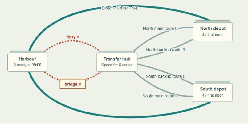
The original plan loses both orders when the bridge and ferry close together. The least-cost plan meets both orders in every case for 17 budget units.
Open the planning toolIllustrative network. The map shows one of the 29 cases.
How Aptifold verifies results
Aptifold picks a check based on what could make the result wrong. A reviewable result shows the criterion, the inputs and assumptions, the expected and observed outcomes, and the conditions under which the conclusion holds.
- Reproduce a reference
- Rework a published result using its data and conventions. In the GW150914 reproduction, five of seven checks matched at first. Two peak times differed until the analysis used the notebook’s window convention. Inspect the two runs.
- Check against an independent calculation
- Use a second route to the answer. The delivery planner checks a feasible dispatch against a capacity bound. A separately written crate-routing calculation checks the totals using the same network assumptions. See the model and checks.
- Use known answers and controls
- Hold the inputs fixed and change the assumption under test. The ringdown comparison uses the same simulated signals and noise draws in each pair. White noise provides a control with a smaller effect. See the experiment and its checks.
- Check that the result serves the brief
- Try a case that could pass the easy test and fail the actual job. A delivery total can pass while one depot gets nothing. Check the end result against the owner’s requirements before they decide to act. Replay the counterexample.
When the data leave two explanations open
Aptifold used early readings of WASP-126 to fit two proposed dimming cycles. It fixed the fitted values before checking the later readings.
- Early readings used to build the predictions
- 390
- Later readings kept back to check them
- 603
The two predictions agreed with each other, so these brightness readings could support either explanation. To choose between them, you would need a new measurement that the two explanations predict differently.
Can you trust a 95% estimate?
A black-hole merger leaves a pattern of fading vibrations, a little like a bell after it’s struck. Researchers filter noisy recordings to measure those vibrations. A well-calibrated 95% estimate should include the true values about 95 times out of 100, when the same test is repeated with fresh noise.
Aptifold made simulated recordings with known answers. In one noise setting, reusing the old noise model captured the true values in 84.5% of repeats. Updating the model for the filtered noise raised that to 94.8%. With plain white noise, both methods came close to 95%.
See the chart, calculation and experimental controls
GRAVITATIONAL-WAVE SIMULATION
How often did a 95% region contain the known answer?
95% target
White noise with a narrow spectral line
White noise alone
Each method quotes a 95% region. We checked whether it held the true values in 2,048 simulations per noise setting. Whiskers show 95% Wilson sampling intervals.
Read the counts and intervals
- White noise with a narrow spectral line
- Reuse the old noise model. 1,730 of 2,048 repeats. Interval 82.8% to 86.0%.
- Recalculate the noise model. 1,941 of 2,048 repeats. Interval 93.7% to 95.7%.
- White noise alone
- Reuse the old noise model. 1,957 of 2,048 repeats. Interval 94.6% to 96.4%.
- Recalculate the noise model. 1,936 of 2,048 repeats. Interval 93.5% to 95.4%.
Reproduce a known result
The agent first used the public GW150914 notebook as a reference. Its implementation matched five of seven quantities, including the delay between the two detectors, while missing both absolute peak times. It traced the discrepancy to how the analysis window was centered. With the notebook’s convention, all seven checks passed. Inspect the two recorded runs.
Make the next question testable
The agent built a two-mode ringdown simulation with fixed, known signal amplitudes. It applied a finite-window filter and reduced the sampling rate from 4,096 to 1,024 Hz. For each noise setting it ran both methods on the same 2,048 noise draws and counted how often the reported 95% region contained all four true amplitude coefficients.
For a linear processing operation H, the original noise covariance Σ becomes HΣH⊤. Covariance captures how noise varies together across samples. The agent compared carrying this transformation into the inference with reusing the old covariance while applying the same processing to the signal in both methods.
Check what the result depends on
In the simulated noise with a narrow spectral line, reusing the old covariance put the known values inside the region in 84.5% of repeats. Updating it raised coverage to 94.8%. With white noise alone, both methods landed near the target. A check using white noise alone would have missed the problem.
These coverage results apply to simulated signals with a known start time and specified Gaussian noise. The separate GW150914 reproduction uses recorded detector data. The research page lets you inspect the models, vary the noise and sampling rate, and see which comparisons the conclusions rely on.
Open the ringdown experimentHow Aptifold learns from work
Aptifold keeps the evidence behind a correction and a test that can catch the same problem again. The lesson records when it applies, so a later investigation can use it when the conditions fit.
Catch the miss
After filtering, the old noise model missed known answers too often in one test.
Keep a test to rerun
Save the signal, the filter, the two noise models and the check against known answers.
Try the lesson in different conditions
Change the kind of noise and run the same comparison. See when accounting for filtering changes the answer.
Compare the results in both noise conditions
| Simulated noise | Original noise model | Updated for filtering |
|---|---|---|
| With narrow interference | 84.5% | 94.8% |
| White noise alone | 95.6% | 94.5% |
The comparison used 2,048 paired trials per noise setting. Explore both settings in the research engine.
The agent built the engines and improved its working methods through the projects on this site. Read how Aptifold carries a lesson into later work.
Paul Wishall founded Aptifold in 2026.
What would you like to investigate or build?
A few sentences are enough to start. Tell us your question, what you already know, and what you’d like to be able to do with the answer.
“Our two models give different estimates. Can Aptifold help us find out why and design a test to decide which one to use?”
Open your email app or copy the address into webmail.
Before work starts, we’ll agree on what you’ll get, how it will be checked and what it will cost.
Explore project possibilities