
Predicting a third wave coupling from two
A rule fixed before a new black-hole calculation predicts its mixed coupling to within 1%. It also suggests a useful way to choose the incoming polarization, with a checked lower-family limit.
Our agent reproduced a published reference, fixed a prediction for a new angular family, then checked it against the calculation. It also worked out what that accuracy permits in the model. The earlier interactive examples below run from recorded couplings in your browser. Read the separate detector investigation ↗
Gravitational waves can mix near a black hole and generate radiation at new frequencies. Three complex couplings describe how the incoming polarizations feed one selected outgoing component. In several examined cases, that response stays close to the square of one linear mixture of the inputs.
Can two calculations predict a third?
In this black-hole model, two incoming gravitational waves interact to produce an outgoing wave. Three complex couplings describe its strength and phase for different input polarization pairs. We used the pure-parity couplings, a and c, to predict the mixed-parity coupling, b. A reliable relation could let model builders calculate two couplings and predict the third.
Predicted b = −a √(c/a)
The new family uses angular-harmonic labels 4 + 4 → 8, which describe directional wave patterns. Frequencies are specified separately. We fixed the rule before running the calculation, computed the pure couplings and recorded the prediction before calculating b. Its baseline complex error was 0.910%. All five numerical variants passed the declared checks. Their observed-variation envelope was 0.891–0.929%; this describes tested numerical variation, rather than a confidence interval or complete error certificate.
| Evidence | Within the 5% criterion | Largest complex error |
|---|---|---|
| New native family · 4 + 4 → 8 | 5 variants · one case | 0.911% |
| Released sample · 3 + 3 → 6 | 89 of 89 frequencies | 1.851% |
| Released lower family · 2 + 2 → 2 | 7 of 88 frequencies | 45.452% |
The released curves supply a wider frequency check and a clear failure. We fixed their predictions before opening the mixed curves and retained every admitted outcome. These frequencies are correlated points in previously examined angular families; the new native case adds a separate angular-family test.
The prediction also has a useful conditional power bound. Holding the calculated pure couplings fixed, substituting predicted b changes selected-family power by at most 1.82% in the new case, over every monochromatic input mixture in its retained variants. The corresponding bound is 3.74% across the retained 3 + 3 → 6 sample. Neither bound certifies physical accuracy at an untested configuration.
This is a bounded empirical candidate. We used the authors’ GR implementation and calculated every coupling to validate the prediction; no avoided solve or speedup was measured. Physical mechanism and scientific originality remain open.
Inspect every retained frequency, the power bound and source coverage
Download the predictions and source values (JSON): all 177 retained source points, the new native case with five variants, branch-control states, source coverage and the three earlier interactive models. Each complex number is [real, imaginary].
The new native case uses identical (4,4) parents at Mω = 0.8 and an (8,8) daughter at 1.6. The five variants change outer radius 4000 → 2000, horizon exponent 5 → 6, quadrature inner exponent 3 → 4, or one allowed counterterm. Flux residuals meet 10⁻⁶; relative outer changes meet 0.005 and other changes meet 0.001. A separate 80-digit reader reconstructs the raw couplings, prediction and numerical decision. These finite checks share the authors’ field-equation solver.
For unit incident parity norm, Ae = a u² − c v², Ao = −2buv and E = |Ae|² + |Ao|². Replacing only b gives |Epred−E|/E = ||bpred|²/|b|²−1| · |Ao|²/E. The last factor reaches one at Ae = 0, so the stated conditional power bound is tight. It concerns the retained couplings and a selected monochromatic family.
Power agreement alone can miss the coupling phase: changing b to −b leaves total-family power unchanged. In an m > 0 family it can reverse axial flux; the selected lower m = 0 family has zero axial flux for either sign. The complex-coupling error therefore remains the prediction test.
The source-curve reader separately checks 177 retained points with 80-digit complex arithmetic. Their admission uses a change between two outer radii, up to 1%, rather than the new native case’s fuller finite-variation checks. This is not a complete numerical-error budget. The six curves belong to the authors’ released scattering data.
Related work already uses factorization of cubic pole residues. Its matrix compares output channels and preparations; it does not establish this incident-parity relation or its physical cause. The square-root sign belongs to the fixed source coordinates. The full physical output retains two comparable response directions.
What can we do with the prediction?
Within this scattering model, the two pure couplings can prescribe an incoming mixture that strongly suppresses one outgoing branch. In the new case, the same chosen input keeps these results across all five numerical variants:
The small remainder follows from an exact relation: at the prescribed mixture, the targeted branch’s power fraction falls quadratically with the complex coupling error. Changing the sign of the input ratio swaps the branches. This describes integrated complex-strain multipoles; their angular pattern remains broad.
The coupling prediction was prospective. This consequence study uses the completed models. The branch percentage, hemisphere power and largest absolute momentum flux are different quantities; scientific originality remains open.
Try the input and angular-distribution controls ↓
Inspect the input rule, full-information baseline and physical limits
Download the branch-control states (JSON): includes both full-coupling baseline roots, every prescribed input, power coefficients and the separate baseline-input stress test.
Set p = v/u = −i bpred/c, u = 1/√(1+|p|²) and v = pu. This state uses only a,c. With H+ = Ae−iAo and H− = conj(Ae+iAo), the targeted fraction is W− = |bpred−b|² / [2(|bpred|²+|b|²)]. For ε = |bpred−b|/|b| < 1, W− ≤ ε² / [2(1+(1−ε)²)]. This bound needs the actual complex-error bound; it does not supply one at an untested point.
| Model check | Targeted branch fraction | Power retained |
|---|---|---|
| New 4 + 4 → 8 case · baseline input held fixed | ≤ 0.0021% | ≥ 95.27% |
| 89 released 3 + 3 → 6 frequencies · a separate prescription at each | Up to 0.008407% | At least about 74.101% |
| 88 lower-family frequencies · a separate prescription at each | Up to 3.31541% | At least about 98.828% |
The illustrative screen requires targeted fraction ≤ 0.1% and at least half of maximum power. Only 9 of the 88 lower-family points meet it. It differs from the coupling-error test. The lower m = 0 family has no axial momentum for any mixture. Knowing all three couplings lets us solve both exact branch-zero roots; in the new base case the better root retains 98.45% of maximum power with an exact zero. The two-coupling prescription instead retains about 95.27% with a small residual.
The identity uses each model’s own a,c prescription. For the numerical stress test we separately hold the baseline p fixed and evaluate all changed models directly. A raw reader reconstructs every state at 80 digits, and real plus/cross news integration checks energy and axial momentum at 16 declared states. The angular relation is Fz/E = [2m/(l(l+1))](1−2W−); its coefficient is 2/9 in the new case. The common physical frequency/strain prefactor is suppressed.
H+ and H− label the positive-/negative-frequency complex-strain multipole branches, with m and −m. The fraction is integrated over angle. Scalar zeros and these angular laws are prior art; this study quantifies the two-coupling prescription’s consequence. It does not establish a new GR interaction, complete order-ε⁴ balance, recoil, observation or a production runtime saving.
When input uncertainty changes the best choice
Making an outgoing branch vanish at one exact input can be a fragile target. We kept six baseline inputs fixed and asked how much that branch could return when the incoming polarization varies nearby, with the same total incident power.
At a 5° polarization-state distance, the two-coupling prescription limits worst-case leakage to 0.01543%. The stronger nominal exact-zero input reaches about 0.03675%; its other root reaches 0.04454%. A separate conservative bound guarantees at least 72.57% of maximum power throughout the two-coupling input’s neighborhood. That is a lower bound, rather than the optimized worst-case power.
The exact zeros still win at the smaller 0.25°, 0.5° and 1° radii. The two-coupling input wins against both at 2°, 3°, 5° and 10°, separately in all five numerical settings. A model builder should therefore compare sensitivity to allowed input changes alongside nominal cancellation.
The degree measure describes distance between normalized even/odd amplitude mixtures. It is not a sky or inclination error, a measured source uncertainty, or a way to tune astrophysical waves. This is one selected monochromatic family; physical cause and scientific originality remain open.
Inspect the tolerance comparison, mechanism and stronger baselines
Download all 240 input-tolerance states (JSON): six fixed baseline inputs, eight radii and five numerical variants, with modal-fraction bounds, power bounds and witness values.
All six baseline inputs at the 5° radius
| Fixed baseline input | Worst branch fraction | Power lower bound |
|---|---|---|
| Pure even | 64.69637% | ≥ 47.38% |
| Two-coupling prescription | 0.01543% | ≥ 72.57% |
| Exact zero · greater nominal power | 0.03675% | ≥ 75.35% |
| Exact zero · other root | 0.04454% | ≥ 68.50% |
| Full-coupling polynomial midpoint | 0.01553% | ≥ 72.34% |
| Maximum power | 0.29762% | ≥ 76.71% |
The full-coupling midpoint performs comparably to the two-coupling input. It is an essential stronger baseline, not a proven robust optimum. This comparison does not show that less information is generally better. Exact zero means exact in the baseline calculation; no input is retuned when the numerical setting changes. The power bounds are conservative and need not be attained at the input that gives the largest leakage.
Why two nearby zeros can help
The unwanted amplitude is a quadratic polynomial. Completing its square gives h−/u² = (ac − b²)/c − c(p + ib/c)², where p = v/u. When b² = ac, its two zeros coincide: a small input error then changes the unwanted amplitude quadratically and its power quartically. Distinct simple zeros give a quadratic leading power error. This standard argument explains a sensitivity effect near the almost-square response. It does not establish why the gravitational couplings nearly satisfy that relation.
The uncertainty cap uses x = cos(η)x₀ + exp(iχ)sin(η)x⊥, with x⊥ orthogonal to the nominal input. It permits every direction of input error up to η = ρ. The maximum-modulus principle reduces the worst-case search to the cap boundary after excluding zeros of the other branch inside. A 32,768-point search has an analytic missing-maximum bound and a separately checked floating arithmetic guard. It is not formal interval arithmetic or a native-coefficient error certificate.
A separate raw reader checks all 240 states at 80 digits, searches 131,072 boundary points for every nonzero-radius row, probes interior states and verifies the derivative and power bounds. All 4,316 checks pass. Both routes share the original native GR coefficients. The radii were fixed before this consequence calculation, but the coefficients and their zeros were already known. This is not a blinded GR prediction, independent field-equation solver, global robust-input optimization, full-radiation calculation or discovery claim.
A harder test · two distinct incoming waves
Three known couplings. One new prediction.
For this chosen pair of incoming gravitational-wave modes, four complex couplings specify the modeled response around a nonrotating black hole. We tested whether three of them could predict the fourth—even when the incoming waves have different angular patterns and frequencies.
Parent 1: ℓ = m = 2, Mω = 0.4.
Parent 2: ℓ = m = 3, Mω = 0.6.
Output: ℓ = m = 5, Mω = 1.0.
Use the three known couplings a, c and bEO. Fix the prediction before calculating bOE.
bOE ≈ a × c / bEOThe missing complex coupling should be:
0.21542 − 0.04749iBoth its magnitude and phase matter.
Reveal the recorded result
0.22079 − 0.05121iAll five numerical settings clear admission.
Scroll the graph sideways ↔
The observed finite-setting envelope is 2.760–3.005%, below the predeclared 5% test threshold. That envelope is a numerical sensitivity diagnostic, rather than a statistical confidence interval or a complete source-error bound.
Why this is a research lead. The result supports a constraint among couplings at this point: the response contains enough structure to predict a calculation we had left out. That could guide a cheaper response model or provide an additional consistency check. Its physical cause and wider range still need testing; no runtime saving has been measured.
Inspect the couplings, numerical controls and open frequency-split test
The same scalar pattern survives independent preparations
The two mixed couplings differ substantially. We therefore use the full bilinear scalar matrix B = [[a, i bEO], [i bOE, −c]], allowing each incoming wave its own normalized even/odd mixture. The small singular-value ratio is 0.006653. The two-row physical response has ratio 0.956445, so both physical output directions remain substantial.
| Entry | Dimensionless complex value |
|---|---|
| Known a | -0.33500 + 0.04579i |
| Known c | -0.18526 + 0.05260i |
| Known bEO | 0.28957 − 0.05734i |
| Predicted bOE | 0.21542 − 0.04749i |
| Computed bOE | 0.22079 − 0.05121i |
| Numerical setting | Coupling error | Scalar σ₂/σ₁ | Physical lift σ₂/σ₁ |
|---|---|---|---|
| base | 2.8827% | 0.006653 | 0.956445 |
| outer | 2.8829% | 0.006653 | 0.956446 |
| horizon | 2.8827% | 0.006653 | 0.956445 |
| inner | 2.8803% | 0.006646 | 0.956335 |
| counterterm | 2.8862% | 0.006661 | 0.956481 |
A finite-boundary control mattered
Swapping the incoming waves initially failed a strict consistency check. A separate differential-operator calculation identified a regularizing field redefinition. Its boundary term explains the discrepancy within the original tolerance; the residual is 3.45e-07 against 10⁻⁶. The prediction itself receives no fitted correction. All original variants and the stopped attempt remain part of the evidence. A separate 80-digit arithmetic implementation checks the completed response and its consequences.
Broader frequency splits remain open
This successful case has equal reduced parent frequencies, ω₁/ℓ₁ = ω₂/ℓ₂ = 0.2. A fixed-output-frequency contrast at 0.25 and 0.75 does not clear the boundary control: its unexplained residual is 1.57e-06 against 10⁻⁶. The fourth coupling stays uncomputed there. That result leaves the frequency-split question unresolved.
These are theoretical monochromatic modes in the published Schwarzschild scattering model. Five settings are variations of one physical case. The separate arithmetic shares the author’s source and linear solutions; scientific priority, full source-error certification and observational usefulness remain open.
Why a small coupling error can still give a poor relative power estimate
Two independent incident mixtures can cancel both selected-family output amplitudes. Replacing one coupling by an approximation shifts that cancellation. Nearby, the true power can be tiny while the approximation remains finite, making their relative difference large.
On a fixed near-cancellation path in this recorded model, a true reduced power of 1.3125e-06 becomes 1.5594e-05 under the substitution—about 11.9 times larger. The absolute difference stays small. A uniform relative-power guarantee would therefore be the wrong promise across all independent preparations.
The model amplitudes are Ae = a u₁u₂ − c v₁v₂ and Ao = −(bEO u₁v₂ + bOE v₁u₂). Their reduced power is |Ae|² + |Ao|², with fixed frequency/angular factors omitted consistently. It is not a value in watts. The roots p₁² = −a bEO/(c bOE), p₂ = a/(c p₁) give two selected-family dark states. They do not cancel the complete radiation field or establish an astrophysical tuning mechanism.
The absolute bound 2‖L‖ |δbOE| + |δbOE|² remains available. Here it is 0.005127 in the same reduced units. The source-values record retains both roots, all five settings and the six fixed approaches to a cancellation.
TRY THE RECORDED MODEL · 4 + 4 → 8
Choose the input. See what leaves.
Mix the two incoming polarizations and compare three different outcomes: which wave branch survives, how much power remains, and where that power goes. The expensive scattering calculations are recorded; these controls evaluate their model locally.
Two-coupling inputUses baseline a and c
The remaining share goes into the odd polarization.
Phase controls how the two responses reinforce or cancel.
Reversal keeps the power and exchanges the two branches.
Try the numerical checks
Your input stays fixed when this changes. Each preset was chosen from the baseline calculation.
of this input’s outgoing power, in the negative-frequency branch.
of the maximum available in the selected calculation.
Positive-frequency branch 99.99791%Negative-frequency branch 0.00209%
Where that power goes
83.38% in the north
The two-coupling input almost removes one branch while keeping most of the available power.
Read the formulas, baselines and limits
The two-coupling prescription uses a and c. “Exact branch zero” and “Most power” also use the calculated mixed coupling, b. These are information requirements: we calculated every coupling for validation and have not measured a saved solve or speedup.
All inputs satisfy |u|² + |v|² = 1. With u real and nonnegative, the controls set |u|² and arg(v/u). The outgoing parity amplitudes are Ae = au² − cv² and Ao = −2buv. The positive- and negative-frequency complex-strain branches have squared magnitudes |Ae − iAo|² and |Ae + iAo|².
Writing W for the negative-frequency fraction, the normalized angular density is (1 − W)f(x) + Wf(−x), where x = cos θ and f(x) = 68068[(1 + x)/2]¹⁰[(1 − x)/2]⁶. This established spin-(−2), l = m = 8 pattern integrates to one. A pure positive-frequency branch puts 54647/65536 ≈ 83.38% of its power in the northern hemisphere, rather than all of it.
Signed axial momentum flux divided by this family’s power is in units with c = 1. It equals (2/9)(1 − 2W); it is not angular momentum or a remnant kick. The graph integrates over azimuth and averages over the monochromatic cycle.
This is one selected second-harmonic family at parent Mω = 0.8, with outgoing frequency Mω = 1.6. It does not model all emitted radiation, a physical source population, detector visibility or complete order-ε⁴ flux. Numerical checks explore recorded settings, not a statistical confidence interval. A baseline zero need not remain exact in another numerical variant.
Download the recorded input states and angular law (JSON). Full-precision preset values, all five coupling triples and independent reference outputs are included.
How the shortcut was identified
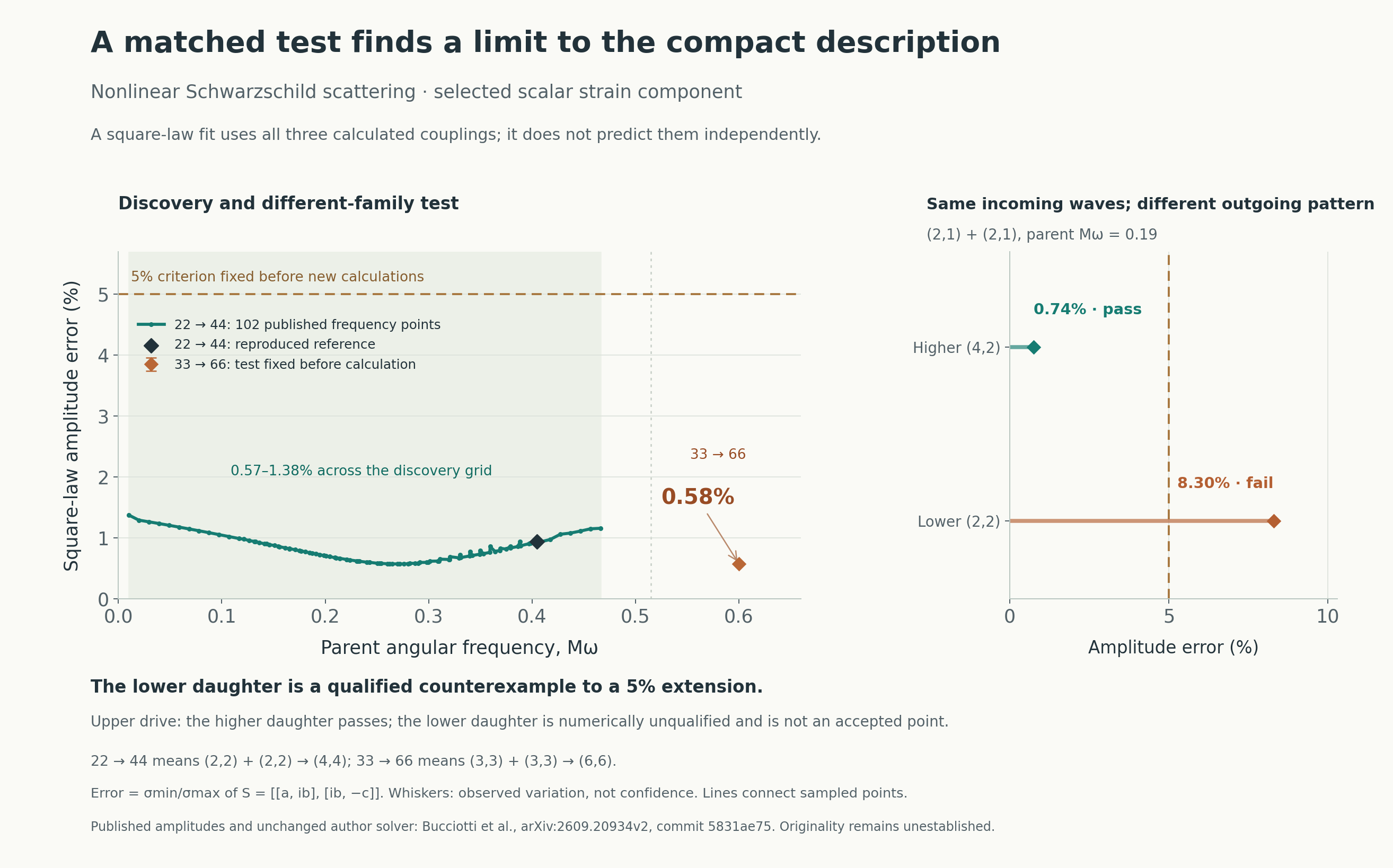
We found the pattern in 102 frequency points released with Bucciotti and colleagues’ scattering calculation. A different-family test, fixed before calculation, returned 0.58% amplitude error. We then kept the incoming waves matched and changed the outgoing angular pattern. The error rose from 0.74% to 8.30%, with both cases passing their declared numerical checks.
Candidate, with a checked counterexample. The result supports a compact description in the examined maximal daughters; it does not support a universal 5% rule. Separate high-precision arithmetic confirms the decisions. The physical cause and scientific originality remain open, and nearby component cancellations are established prior work.
| Evidence | Amplitude error | What was tested |
|---|---|---|
| Matched higher pattern | 0.74% · pass | (2,1) parents → (4,2), parent Mω = 0.19. |
| Matched lower pattern | 8.30% · fail | Same parents and frequency → (2,2). Fails the fixed 5% approximation criterion. |
| Published discovery grid | 0.57–1.38% | 102 shared frequencies; one 22 → 44 family. Exploratory analysis. |
| Different-family test | 0.58% · pass | 33 → 66 at Mω = 0.6; criterion fixed before this calculation. |
| Upper-drive higher pattern | 0.94% · pass | (2,1) parents → (4,2), Mω = 0.404589. Known scaling check also passes. |
| Upper-drive lower pattern | Unqualified | Inner-cutoff and counterterm checks fail. No accepted error value or frequency-trend claim. |
Why this is worth investigating
A reduced scattering model needs an error check for each outgoing pattern. Testing more frequencies in the original pattern would have missed this counterexample. The difference cannot come from a common amplitude rescaling: that leaves the error ratio unchanged. The outgoing angular source and radial propagation both change, so this experiment does not yet identify the cause.
That initial native transfer predicted a property of the response. We still calculated all three couplings before fitting the square-law form; no GR calculation was avoided.
Explore the earlier scalar approximation
These controls use the full calculated couplings for the earlier three cases. The new 4 + 4 → 8 prediction and branch prescription are separate calculations. Switch between the matched outgoing patterns while keeping the incoming mixture and phase fixed. The directional chart shows where this selected wave family sends its power. “Show largest mismatch” selects an input that reaches the current case’s worst approximation error; the component comparison remains available below.
Worst amplitude error for this case: %.
Complex-amplitude difference: % of that reference scale.
Selected-family power: % of its largest response.
Axial directed flux: % of max ·
Directed flux uses this family’s greatest possible magnitude as 100%. Northward and southward values have opposite signs. Power and flux use the full calculated wave components.
Area under the curve gives this family’s share of power. Equal horizontal steps cover equal-solid-angle bands; the left half is south and the right half is north. Each selected family totals 100%.
Arrow keys change an angle by 1°; Shift + arrow changes it by 5°. Total incoming power stays fixed.
Compare the calculated and fitted wave components
Bar lengths show amplitude relative to this component’s strongest possible response. They are not power percentages.
The real wave includes both components. A compact fit can miss a weak component while the other still carries strong radiation. Inspect the complex-amplitude difference separately from the selected-family power.
Each case has its own amplitude scale; the bars compare approximation quality rather than radiation strength across cases. A small global amplitude error does not promise a small relative error at a cancellation. The total selected-family power includes both real-wave components.
Most radiation, or most directed momentum?
For the matched higher pattern, pure-even input produces the most power and zero net momentum along the chosen axis. A mixed input keeps 83.9% of that power while maximizing northward momentum flux. Reverse its relative phase by 180° and the flux points south at the same power.
Try “Most power,” then “Max northward flux.” Watch the two readouts together. In the lower pattern, the power-maximizing input already reaches 99.99% of maximum directed flux. The tradeoff depends on the outgoing pattern.
Axial momentum weights the radiation by its direction, cosθ. It differs from simply counting the power in each hemisphere. This is one selected second-harmonic contribution; a complete recoil calculation also needs the other radiation, the incoming drive and higher-order interference.
Does that tradeoff survive the combined radiation?
Almost none of it survives in this case. The same incoming wave drives both the lower and higher patterns. When we combine them using one common input, the lower pattern dominates. The input that sends the most axial momentum north keeps 99.65% of the available power.
| Choose the input for | Combined power | Axial-momentum magnitude |
|---|---|---|
| Most power | 100% | 99.55% |
| Most northward momentum | 99.65% | 100% |
Each column uses its own attainable maximum. We cannot add the best result from each pattern: those separate optima require different incoming mixtures. A striking effect in one pattern can become small when the whole output enters the calculation.
This result covers the forced, twice-frequency radiation from the stated single traveling (2,1) drive, including both real-wave partners. It excludes zero-frequency content, incoming momentum and higher-order interference, so it still does not give a black-hole kick. The controls above continue to show each pattern separately.
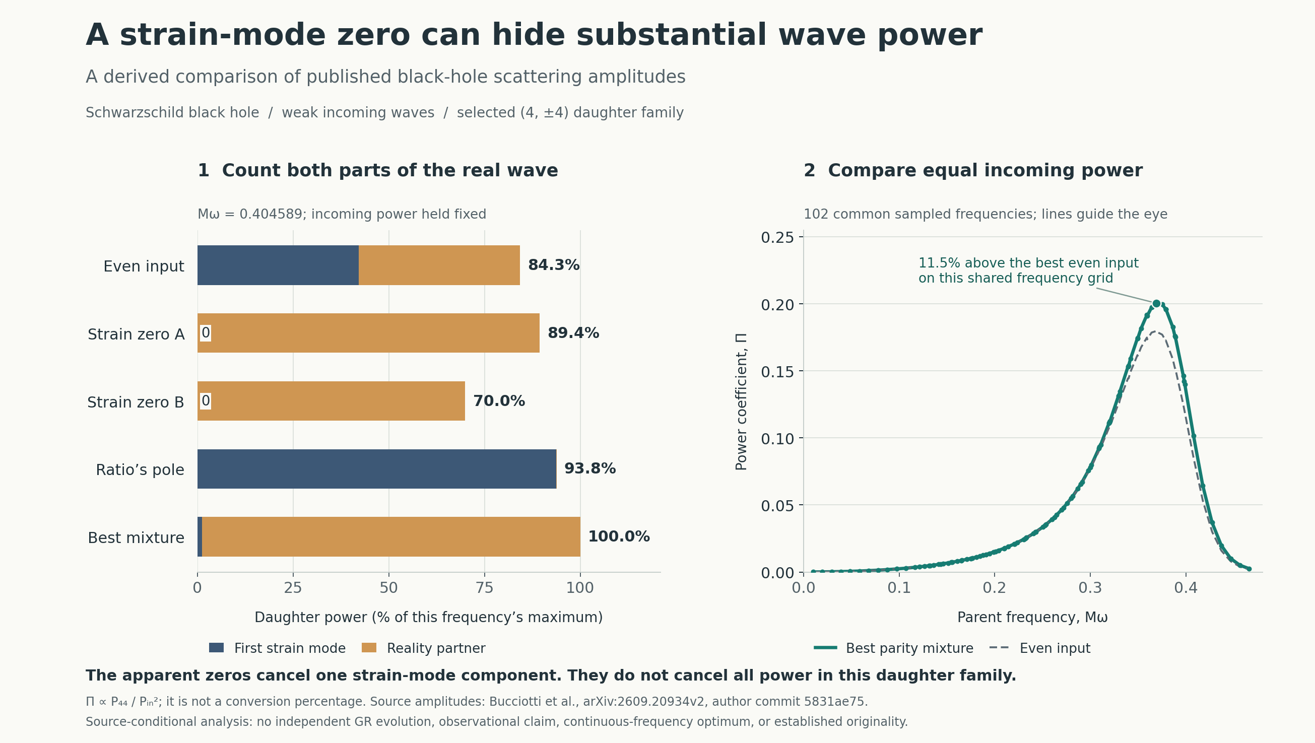
The cancellation can leave strong, directional radiation
In the published reference model, the two input mixtures that cancel the plotted component retain about 89% and 70% of the strongest selected-family power at that frequency. The reality partner carries the remaining radiation. A separate angular integration confirms that these states send about 9% of this family’s power north and 91% south, where north means cosθ > 0 on the chosen +z harmonic axis. Changing the sign of the input parity ratio reverses the imbalance.
That directionality follows from established wave-flux laws applied to these coefficients. It is not a computed black-hole recoil: a recoil calculation needs the complete incoming and outgoing momentum balance and the remnant response.
Inspect the mathematics, controls and scope
Download the model inputs and predictions (JSON): the three earlier interactive cases, source-frequency predictions, new native case and branch-control states. Complex numbers use [real, imaginary].
Let x = (u,v) contain the incident even/odd amplitudes with |u|² + |v|² = 1. For matched incident-normalized couplings a = Qeee, b = Qeoo, c = Qooe, one outgoing scalar component is
H+ = a u² + 2 i b u v − c v² = xᵀ S x,
S = [[a, i b], [i b, −c]].
The best symmetric rank-one approximation has the square-law form κ(w₁u + w₂v)². Its worst absolute amplitude error, relative to the component’s maximum response, is r = σmin(S) / σmax(S). Unitary changes of the input basis preserve this ratio when they preserve the incident-power norm. It is not a uniform relative-error guarantee at every input.
The direction view uses spin-weight −2 spherical harmonics for the selected (l,m) pair. Its horizontal axis is x = cosθ from −1 to +1, and its height is the normalized time-averaged power density d(P/Pfamily)/dx. Equal x steps cover equal solid angle after integrating the azimuth. The fixed vertical scale runs from 0 to 4.5; the area under each curve is one. North means x > 0 on the chosen +z axis. Combining different families requires their interference terms; these separately normalized distributions are not a complete all-mode emission model.
Power and directed flux solve different optimizations
For this one (l,±m) family, the established axial linear-momentum law gives Fz = [2m/(l(l+1))] (|H+|²−|H−|²)/2 = k E D, with E = |Ae|²+|Ao|². Signed Fz weights the outgoing energy by cosθ. The displayed flux percentage is Fz divided by this family’s own maximum magnitude, which differs from its energy maximum and from the hemisphere percentages.
Let f be the incident even-power fraction: u=√f, v=√(1−f)eⁱᵠ, α=a b*, β=c* b. Then Fz=4k√[f(1−f)] Im[(αf+β(1−f))e⁻ⁱᵠ]. Maximizing the phase leaves a quartic in f; its endpoints and real stationary roots supply the global maximum. A separate optimizer searched the original complex outputs, and time-dependent real-news sphere integration checked the angular result.
The higher pattern’s directed optimum retains 83.9% of maximum power. Its power optimum stays pure even with zero axial flux in every retained numerical variant. The lower pattern’s power optimum reaches 99.99% of maximum directed-flux magnitude. These are finite-model results at the stated drive. The selected second-harmonic squared-news contribution is order ε⁴; other outgoing families, the incoming field and first/third-order interference matter to a complete calculation. The optimized incoming field can carry momentum itself.
One input for both outgoing patterns
For the traveling (2,1) drive at Mω = 0.19, the common Wigner factor makes the (3,2) daughter vanish; only (2,2) and (4,2) radiate at 2ω. Their energy and axial momentum add at a fixed common input because full-sphere orthogonality removes the energy cross term and cosθ couples only equal or adjacent angular degrees. Their local angular intensities and hemispheric powers still interfere.
Set A=Σ|aⱼ|², B=Σ|bⱼ|², C=Σ|cⱼ|², T=Σaⱼcⱼ*. The common-input power envelope is A f²+C(1−f)²+(4B+2|T|)f(1−f). The flux envelope uses αΣ=Σkⱼaⱼbⱼ* and βΣ=Σkⱼcⱼ*bⱼ in the same quartic calculation. A separate search of the original complex outputs and coherent real-news integrals pass 105 checks. All five retained numerical variants keep both objective losses below 0.5%. This narrows the interpretation of the selected-pattern tradeoff without changing it.
The opposite-frequency partner must remain in the real metric. Its quadratic form uses P S P, with P = diag(1,−1), followed by conjugation. The full parity output acts on (u², √2uv, v²) through L = [[a,0,−c],[0,−√2b,0]]. This is a different object. In the 33 → 66 case its two singular values have ratio 0.972, so the small scalar ratio does not justify a one-channel full physical response.
The prospective test
We fixed the 33 → 66 case at parent Mω = 0.6 and the 5% criterion before calculating its coefficients. The resulting reference values are shown below; their printed digits preserve numerical outputs, rather than establish an equivalent accuracy guarantee.
| Coupling | Incident-normalized value |
|---|---|
| a / eee | 0.19379653 -0.0321400948 i |
| b / eoo | -0.158243831 +0.0353956288 i |
| c / ooe | 0.125970428 -0.0349773492 i |
The declared checks varied the outer domain, horizon starting radius, quadrature cutoff and one subleading counterterm. Every numerical gate passed; the largest relative coefficient change was about 0.0271%. The observed matrix-variation envelope gives r between 0.56–0.60%. Its upper endpoint is below 5%, so the predefined refinement was unnecessary and was not run.
A separate 80-digit Decimal implementation reconstructed the singular values and decision from all 15 raw numerical records. It passed 165 checks. Both routes share the author’s GR implementation; independent arithmetic does not independently validate those field equations or supply a comprehensive error bound.
What existing work may explain
The scattering paper already shows nearby scalar roots. Related QQNM parity work and chiral coupling classifications provide a self term and a weaker mixed term that can naturally yield a small second singular value. Their application to these real-frequency incident states needs an explicit boundary-state mapping.
As an exploratory diagnostic, neither a single-parity projection nor simply deleting the weaker circular-input diagonal gives a 5% approximation on 73 of the 102 discovery rows. The fitted square-law description still does. That comparison does not identify a new mechanism or exclude known physics after the correct state mapping.
A later check includes the established Darboux reflection phase. For the lower-drive higher pattern, the best scalar rank-one error remains 0.74%, while deleting either squared term in that specified outgoing basis costs at least 9.45%. The phase change preserves intrinsic compactness. This excludes one missing-square approximation; a bulk QNM-to-scattering mapping and scientific originality remain unresolved.
The matched contrast and its unresolved cell
The four-cell contrast was fixed before calculation. At parent Mω = 0.19, the lower-pattern error lies in the observed-variation range 8.29665–8.30072%; the higher-pattern range is 0.73791–0.73909%. These disjoint finite envelopes support a difference at that drive. At the upper drive, the lower pattern failed the fixed numerical checks: inner-cutoff variation reached 0.609% and counterterm variation reached 0.141%, above the 0.1% criterion. Its small raw estimate is not an admitted result.
A separate 80-digit calculation agrees on all four decisions in 257 checks. The known common-m scaling also reproduces the upper-drive higher pattern within 0.00036%. We have not established a frequency trend for the lower pattern, a universal angular law, or a state-matched physical explanation.
Current claim. A compact scalar description works in the examined maximal daughter families and fails the 5% criterion in one qualified lower daughter. One additional cell remains numerically unqualified. This is a bounded research lead with a counterexample, not established new physics, scientific priority or an observational application.
Primary sources: Bucciotti et al., second-order scattering; exact published reference coefficients; pinned MIT author code; Ruiz et al., energy and momentum flux; strain and reality-partner conventions.
Updated after the native reference, different-family and matched daughter checks, 1 November 2026. Working analysis; scientific originality and physical mechanism remain open.