
GRAVITATIONAL WAVES / CHECKING THE ANALYSIS
How reliable is
a black-hole estimate?
A black hole’s fading gravitational waves help physicists estimate its mass and spin. To test gravity with those estimates, they need uncertainty they can trust.
Our agent reproduced a public LIGO analysis, then tested uncertainty with simulated signals whose true values were known.
Read the gravitational-wave scattering study
The observations are real; the uncertainty experiments are simulated. The controls inspect saved calculations.
WHAT THE AGENT FOUND
Check the result.
Test its uncertainty.
The agent checked its calculation against a published reference, then used simulated signals with known answers to test its uncertainty. The two tests reveal different ways an analysis can go wrong.
01 / REAL DETECTOR DATA
A matching time gap hid two wrong times.
- Earlier run
- 5 / 7
- Corrected run
- 7 / 7
Declared notebook checks matched
Both calculated peak times were late, even though their gap matched. The agent corrected which timestamp it used to select the data; all seven checks then matched. Checking only the gap would have missed the error.
Compare the two saved runsThis repaired the agent’s reproduction, not LIGO’s observations or notebook.
02 / SIMULATED RINGING SIGNALS
A “95%” region missed the truth too often.
- Match signal only
- 84.5%
- Match signal + noise
- 94.8%
Repeats including all four known values · 95% target
A 95% procedure should include the known values in about 95% of repeats. In 2,048 simulations, keeping the old noise description missed that target; updating it along with the signal brought the result close.
Inspect the 95% testJoint regions for four fitted signal amplitudes, not measured black-hole mass and spin. Shown: 1,024 Hz, white noise plus a narrow line.
Email us about a result you’d like checked
New to this? Three ideas behind the investigation
- Ringdown
- The fading gravitational-wave signal as the newly merged black hole settles. Its frequencies and decay rates carry clues to mass and spin.
- Filtering
- A mathematical operation on the data, used here while reducing the number of samples. It changes the signal and the pattern of the noise together.
- A 95% confidence region
- Repeat the experiment with the same true signal and fresh noise. A calibrated 95% procedure should include those true values in its quoted region about 95% of the time. That’s what the four-amplitude test measures.
Start with a signal
the world already knows.
In 2015, LIGO’s Hanford and Livingston detectors recorded GW150914, a signal from two merging black holes. The two instruments saw it a few milliseconds apart. The discovery belongs to the LIGO and Virgo collaborations.
Our agent used their public teaching notebook as a check on its own implementation. It compared seven outputs: two peak times, two signal-to-noise ratios, and three relationships between the detectors. The observations, template, method and reference numbers came from the original scientific work.
Try the detector controls first, then compare the agent’s two saved runs. The later simulations ask a different question: when a method quotes uncertainty, does it hold up against a known answer?
01 / FIND THE SIGNAL
A shape emerges
from the noise.
A matched filter slides a predicted waveform across the observations and scores how well they line up. Frequencies with louder noise count less. The score rises sharply near the signal in both detectors.
Drag across the chart to compare both detectors at the same moment, or use the time slider below. Their peaks are close, but they don’t coincide.
Template-match score · SNR
Time in seconds after GPS 1126259462
- Time after GPS 1126259462
- +0.453125 s
- Hanford · H1
- 5.046 SNR
- Livingston · L1
- 13.391 SNR
The discrete peaks are 29 samples apart: 7.080078125 milliseconds. These times follow the supplied template’s convention; they are not a new estimate of the merger time.
Recorded output of the corrected calculation · 4,096 samples/second · This is a filter score, not the raw detector waveform or a false-alarm probability.
How the filter gives different frequencies their weight
The calculation compares the data d with a supplied template h in the frequency domain. It weights their product by the inverse noise power spectrum Sn, then transforms back to a score over possible time offsets.
z(t) ∝ ∑k [d̃k h̃k* / Sn,k] exp(2πi fkt)
The magnitude of this complex output, divided by the template’s noise-weighted normalization, gives the plotted signal-to-noise ratio. The noise spectrum comes from a 1,024-second interval, using overlapping four-second Tukey-windowed segments. This teaching calculation uses a supplied template. The original discovery used much more: independent searches, waveform families, noise checks and statistical background comparisons.
The downloaded record keeps all 16,383 points from each detector. Download the curves and follow-up record · JSON ↗
02 / CHECK THE RESULT
Five checks passed.
Two still mattered.
Select a run. Compare each detector’s timing error, then inspect all seven quantities. The controls show saved results; they do not rerun the analysis.
On a small screen, scroll the table sideways to compare the notebook, recorded result, and check.
Analysis-window center
1126259462.4GPS seconds
The detector-to-detector delay matched. Both absolute peak times missed.
| Quantity | Notebook | Recorded result | Check |
|---|---|---|---|
| Hanford peak time | +0.460200 s | +0.860107 s | × Outside |
| Livingston peak time | +0.453100 s | +0.853027 s | × Outside |
| Hanford signal-to-noise ratio | 19.0000 | 19.0864 | ✓ Matched |
| Livingston signal-to-noise ratio | 13.4000 | 13.3320 | ✓ Matched |
| H1 minus L1 phase | -2.92000 rad | -2.91868 rad | ✓ Matched |
| H1 minus L1 peak-time delay | 0.007080000 s | 0.007080078 s | ✓ Matched |
| H1 / L1 signal-to-noise ratio | 1.42143412 | 1.43162753 | ✓ Matched |
H1 is Hanford; L1 is Livingston. Peak times are shown as seconds after GPS 1126259462. SNR is dimensionless. “Matched” means inside a declared interval, not exact equality; all intervals and full-precision GPS values are available below.
The earlier run is shown above. The complete comparison is available in the downloadable results below; the switch needs JavaScript to finish loading.
Both times shifted.
Their gap stayed put.
The earlier run recovered the roughly 7.08-millisecond gap between detectors. Yet both absolute peak times were about 0.4 seconds late. Moving two points together can leave their separation unchanged.
The agent had used the catalog event time, 1126259462.4, where the notebook uses 1126259462 to select the analysis window. Both are GPS timestamps. They serve different roles.
Restoring the notebook’s window-center convention brought all seven results inside the acceptance intervals fixed before that run. A repeated execution produced byte-identical numerical output.
Why this matters: several correct-looking results can survive a wrong input convention. A useful reproduction checks what each input means, as well as what the final numbers look like.
The mismatch arose in our agent’s reproduction. It was not an error in the LIGO observations or the published notebook.
03 / A FOLLOW-UP QUESTION
Which frequencies
move the answer?
The noise estimate changes how much weight each part of the data receives. Does that move the best-match time? Our agent derived the response to a small change, then checked it by recalculating seven frequency bands.
Choose a frequency band, then try “Every frequency equally.” A uniform rescaling changes the score without moving its peak. A change in one band can move the peak, and the detectors needn’t respond alike.
Local linear prediction for a 0.1% rise in the band’s noise power · nanoseconds
A 0.1% rise in estimated noise power from 200–350 Hz gives a local prediction of 33.96 nanoseconds more H1−L1 delay. This is a very small response in this fixed calculation.
One sample spans about 244,141 ns. These predicted shifts are much smaller. This is numerical sensitivity to a specified change, not a measured clock shift or statistical timing uncertainty.
Inspect the derivative, checks and scientific limits
Write the unnormalized complex filter as z(t) = ∑ ck exp(iωkt) and its peak power as Q = |z|². Change log noise power by εqk, so the filter coefficients become ck exp(−εqk). Implicit differentiation of the stationary-peak condition gives:
dt*/dε = 2 Re[z′q z* + z′ z*q] / Q″
Here zq inserts the selected frequency weights into the same sum. The filter’s overall normalization is constant across time, so it changes the score’s scale without changing the peak’s location. This derivative needs an interior, nondegenerate local maximum. A flat peak or a switch to a different winning peak can invalidate the prediction.
Both detector baselines exactly matched the earlier recorded calculation. All 28 declared finite-change checks passed, at ε = ±0.001 and ±0.0005 across seven bands. The slope tolerance was 10⁻⁹ seconds plus 0.001 times the absolute analytic slope. An independent interpolation of the original filter power agreed with the local peak positions within a separately declared 10 ns numerical check.
The sensitivity uses a continuous interpolation of the fixed filter. It keeps that quantity separate from the discrete 29-sample notebook comparison above. Neither supplies an astrophysical uncertainty estimate. That would also require justified uncertainty in the noise spectrum, template, calibration and inference model.
This is a new follow-up calculation in this case study. It does not establish a novel method, a new gravitational-wave detection or an additional black-hole vibration mode. The broader scientific investigation remains open.
Full-precision band slopes · CSV ↗04 / SYNTHETIC FOLLOW-UP
Does “95%”
hold up?
Our agent simulated signals with known amplitudes and repeated the analysis with fresh noise. A calibrated 95% procedure should include those fixed, true values in its quoted region in about 95% of repeats.
Select “Match the signal only,” then “Match signal and noise.” Compare their percentages with the 95% target. These are joint regions for four signal amplitudes in simulated ringing signals, not new LIGO measurements.
Coverage over 2,048 repeats · select a method
│ 95% target · whiskers: 95% sampling interval1,730 of 2,048 repeats contained the true four amplitudes in the quoted 95% joint region. The signal operations now match. But removing the surrounding data also removed its noise contribution; this route keeps the old covariance.
Recorded ensemble: 2,048 paired draws per noise model · raw SNR 80 · phase 0.3 rad · four amplitude quadratures. The target is 95%; making a region needlessly broad can push coverage higher while losing precision. Controls inspect saved cases.
Would a stronger signal fix the mistake?
Same analysis. Two known signal strengths.
Choose a mistake to inspect. Raw SNR measures the known synthetic signal’s strength relative to the noise before processing. Both rows use the selected noise setting and sampling rate.
White noise + a narrow line · 1,024 Hz · phase 0.3 rad
Recorded joint-region coverage · 0–100%│ 95% target
1,730 of 2,048 repeats · 95% sampling interval for this fraction: 82.8–86.0%
1,730 of 2,048 repeats · 95% sampling interval for this fraction: 82.8–86.0%
Processing changed the retained noise. This method still uses the old covariance to draw its error region. Turning up the signal leaves that noise mismatch in place.
What information did the filter give up?
- Linear-study amplitude direction
- 68.7% information retained
- Approximate-Kerr mass/spin direction
- 89.3% local information retained
- Sample rate
- 1,024Hz, from 4,096
Each study compares its own model with its exact raw-window likelihood. The approximate-Kerr study below uses slightly different mode frequencies and decay rates. Its mass/spin values describe expected local Fisher information after allowing free amplitudes. A single posterior’s width can behave differently.
Why the noise has to move with the signal
Filtering a full record can mix the surrounding merger signal into a short ringdown window. Subtract that exterior contribution and the retained observations become Td, where T is a finite-window operation. Apply the same map to the model, Th, and to the covariance, TCTT. Keeping the old stationary covariance describes noise that has partly been removed.
The line case’s “match the signal only” route has an independently calculated coverage probability of about 83.77%, consistent with the recorded 84.47% at 1,024 Hz. The paired route restores calibration under the declared Gaussian model, while giving up information. This implements one window-local approach of the kind discussed as future work in Siegel, Isi and Farr’s conditioning study. Existing gating and inpainting methods already recover the truncated likelihood; novelty and an advantage over those methods remain open.
The wider study includes 24 fixed combinations: two noise models, three rates, two phases and SNR 20 or 80. Fifteen mechanism tests cover the numerical operations, likelihood identities and marginalized model. A scoped check reproduces the native ringdown software’s numerical filtering to better than 1.2 × 10⁻¹⁵ relative error. That check does not qualify its complete Bayesian pipeline.
05 / LET THE PHYSICAL PARAMETERS VARY
What black hole
would you infer?
How would a processing choice change the black hole you infer? The agent varied the model’s mass and spin, integrated over four unknown signal amplitudes, and compared the resulting posterior regions. Each posterior describes which values the data and stated assumptions support.
Physicists compare ringing components to check whether one black hole can explain them. The cross marks the known synthetic truth here: 68 solar masses and spin 0.69. Inner and outer contours enclose 68% and 95% of each posterior. The table shows the means. Zero KL divergence means identical grid posteriors; larger values mean more change.
Detector-frame mass · nominal solar masses
| Analysis | Mass | Spin | Difference from raw KL divergence · nats |
|---|---|---|---|
| Raw-window reference | 68.65 | 0.680 | 0.000 |
| Match signal and noise | 68.74 | 0.690 | 0.108 |
| Data and model differ | 65.32 | 0.629 | 1.215 |
With a narrow noise line and this fixed noisy observation, the paired and raw posterior means differ by 0.09 solar masses and 0.010 in spin. The regions show what each declared model supports. Noise, lost information and amplitude priors can change their shapes.
Separate physical-parameter study: the same approximate two-mode family generates and fits the signal. One preselected noisy observation per noise model; no posterior-coverage claim. The browser inspects recorded posteriors and does not run a new analysis.
Change the assumptions before trusting the interpretation
Mass and spin are uniform on 55–85 nominal solar masses and 0.4–0.9. Four real quadrature amplitudes have independent, zero-mean Gaussian priors. The contours fix their standard deviation at 50 normalized strain units. The table below shows what happens when that scale is 25 or 100 instead; it updates with the selected observation.
| Analysis | Prior scale | Mass | Spin |
|---|---|---|---|
| Raw-window reference | 25 | 70.96 | 0.718 |
| Raw-window reference | 50 | 68.65 | 0.680 |
| Raw-window reference | 100 | 68.08 | 0.670 |
| Match signal and noise | 25 | 70.49 | 0.716 |
| Match signal and noise | 50 | 68.74 | 0.690 |
| Match signal and noise | 100 | 68.32 | 0.684 |
| Data and model differ | 25 | 66.54 | 0.648 |
| Data and model differ | 50 | 65.32 | 0.629 |
| Data and model differ | 100 | 65.03 | 0.625 |
For the noisy line case, the raw mean mass moves from 70.96 to 68.08 as that prior scale increases from 25 to 100. The largest true quadrature is about 99 units, making the 25-unit prior restrictive. The interpretation must carry that assumption with it.
The model uses published fits to the (2,2,0) and (2,2,1) Kerr mode frequencies and quality factors. Their reported maximum fit errors are percent-level. Grids of 61 × 51 and 121 × 101 points passed the declared convergence and boundary checks under all three amplitude-prior scales. Agreement between an injection and the same approximate model is a numerical control, not a validation of general relativity.
The amplitude integration is analytic. With F = MTK−1M, t = MTK−1y, and A = I + σ²F, its log likelihood is −½ log det A + ½σ²tTA−1t, plus a term constant in mass and spin. A direct Gaussian-covariance calculation independently checks this expression.
The exact raw acyclic likelihood is the strong reference. Established time-domain inference, inpainting, and sufficient-statistic compression remain relevant alternatives. This experiment establishes no new vibration mode, improved real-event measurement, or novel method.
Do the mass and spin posteriors calibrate across simulated systems?
Test the procedure across known systems.
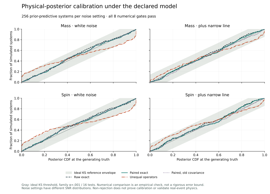
One posterior plot describes one observation. We also drew 256 systems from the stated priors, simulated their signals and noise, and checked the resulting mass and spin probabilities.
This is a separate experiment from the fixed-amplitude confidence regions above. It uses uniform mass and spin priors and a Gaussian prior for four unknown signal amplitudes.
Mass · white noise · 256 systems · median optimal SNR 149.82
Posterior quantile of the known mass
The different-operator route crosses the declared threshold for mass in this white-noise ensemble. The other routes are not flagged by this test.
Scroll the table sideways on a small screen.
| Analysis | 95% count | KS distance | Reference p | Grid change | Declared result |
|---|---|---|---|---|---|
| Raw exact | 240/256 (93.8%) | 0.05856 | 0.331 | 0.00433 | Not flagged |
| Paired exact | 241/256 (94.1%) | 0.05024 | 0.521 | 0.00337 | Not flagged |
| Different data/model operations | 169/256 (66.0%) | 0.16751 | 9.52e-7 | 0.00482 | Flagged |
| Paired signal, old noise model | 241/256 (94.1%) | 0.05832 | 0.336 | 0.00320 | Not flagged |
The ideal KS threshold is 0.14143: family α = 0.001 across 16 mass/spin tests. A flag also requires the distance minus the observed numerical CDF change to exceed that threshold. Counts are descriptive; they do not replace the declared test.
How to read the curves and the test
For each simulated system, we know the true mass and spin. We ask where that value sits in its fitted posterior. For example, a quantile of ½ means half the posterior probability lies below the known value.
With correctly computed posteriors under the stated model and priors, these quantiles should be uniform across repeated systems. The chart compares their accumulated frequency with that diagonal reference. Gray shows the ideal KS envelope, before the additional numerical sensitivity check.
All eight method/noise combinations passed the original numerical thresholds on grids with 269 × 261 and 537 × 525 nodes, concentrated near the prior boundaries. An earlier uniform-grid experiment failed its numerical gate and was retained before this recovery. Independent checks recomputed all 16 statistics and tested an analytic posterior close to a boundary.
Coarse/fine agreement is empirical evidence, not a rigorous uniform error bound. Ideal reference p-values assume exact CDFs. Non-rejection can reflect limited power or errors these marginal tests miss.
Model, priors and limits
Mass: uniform from 55 to 85 nominal solar masses in the detector-frame model. Spin: uniform from 0.4 to 0.9. Four independent amplitude quadratures: Gaussian, mean zero, standard deviation 50 in normalized signal units. Published approximate Kerr fits specify two damped components. The noise covariance and signal start are known.
The same amplitude prior gives different SNR distributions: median 149.82 in white noise and 60.03 with the narrow line. The selector changes both spectral shape and the resulting SNR; it does not compare the methods at a fixed SNR. The methods share generating parameters and paired noise within a setting.
We checked how the inference behaves under the stated model and priors. A real-event analysis also has to test its waveform, noise model, priors and choice of signal start.
Calibration principle: Talts et al., simulation-based calibration ↗. Physical approximation: Berti, Cardoso and Will, approximate Kerr fits ↗.
Do the ringing strengths have reliable uncertainty?
Check another part of the inference.
Mass and spin determine the tones in this model. Four more coefficients set how strongly they ring and where each cycle starts. A method can misjudge the uncertainty in those coefficients, too. Claims about a weak extra ringing component need trustworthy uncertainty in these quantities.
Here we hold mass and spin at known values. That isolates one part of the problem. We check a region for all four coefficients together, across amplitudes drawn from their Gaussian prior and repeated noise.
A region labelled 95% should contain all four true coefficients together 95% of the time in this population. The chart asks whether each method keeps that promise.
At 68 nominal solar masses and spin 0.69, with the narrow-line setup, the old-covariance region covers 83.8% of the stated population. Processing signal and noise together gives 95.0%. Each region claims 95%.
Calculated population coverage · 0 to 100%│ 95% target
The vertical marks show the 95% target. These are calculated probabilities, not counts from a finite simulation. “Variance left” is the reported covariance trace as a percentage of the prior trace, in the same four-coefficient basis.
The method that ignores the observations also gets 95%. It keeps all of its starting uncertainty. Correct coverage alone cannot tell us whether an analysis used the data.
How can a similar total variance hide a wrong uncertainty?
In this coefficient basis, the old-noise calculation reports 4.9% less total variance than the paired calculation. Across the four coefficient combinations, actual error standard deviation (SD) ranges from 0.93× to 1.69× the reported SD. The total hides that unevenness.
Actual error SD ÷ reported SD · all four directions
The outlines show covariance shape at radius 1 in two of the four standardised coefficient directions. Each setting has its own directions and reported-SD units. The coverage above uses all four dimensions.
A value above 1 means the actual error varies more than the reported uncertainty allows. Below 1 means it varies less. These four ordered directions combine the amplitude coefficients; they are not four physical modes. Their meaning can change with the selected mass, spin, noise and reporting method.
Does correcting the noise improve the estimate, too?
Correcting the noise changes how the calculation weights the observations. That can improve the estimates as well as their uncertainty.
At 68 nominal solar masses and spin 0.69, with the narrow line, keeping the old noise produces 40.1% more mean squared coefficient error. Both methods receive the same observations.
Mean squared coefficient error · first row = 1
The two rows use identical observations and the same prior. Change the settings to compare another recorded case. Errors average over the stated amplitude prior and noise.
Under the stated known-noise model, the estimate from processed data has 14.8% more mean squared error than a correct analysis of the unfiltered window. Both rows above compare the same processed observations.
Changing only the error bars leaves these estimates untouched. Even an oracle that gave both methods 95% population coverage would leave their estimation errors as shown. Honest uncertainty and good estimates need separate checks.
Loss, optimality and the limits of this comparison
Let P = 50² I be the four-coefficient prior and R the actual error covariance. The chosen loss is ρ = tr(P⁻¹ R) / 4. Ignoring the observations gives ρ = 1. The plotted ratio divides each loss by the loss with signal and noise processed together at the same setting. The download retains both absolute losses.
For the actual design H and noise C, S = H P Hᵀ + C and G* = P Hᵀ S⁻¹. Any fixed linear estimate G y satisfies R = V* + (G − G*) S (G − G*)ᵀ, where V* is the true conditional covariance. The second term is the extra error shown above. This is established conditional-mean theory.
The loss stays invariant under a consistent invertible linear change of coefficients and prior; the chosen prior and quadratic loss still matter. At the default setting, 40.1% more mean squared error means 18.4% more RMS error, not 40.1% more RMS error.
An oracle region using R would achieve 95% coverage across the Gaussian population without changing G. It is generally not a Bayesian posterior region conditional on one observation, and true R is generally unavailable. This is a thought experiment, not a practical repair.
The post-hoc follow-up checks all 90 methods and 18 same-observation pairs through two numerical formulations. Here mass, spin, onset and noise covariance are known. Unequal data/model operations receive different observations, so they are excluded from this paired comparison. Unknown mass/spin, a real detector signal and mode significance require further work. The earlier inconclusive integral checks remain unchanged.
All 18 error comparisons, loss definition and limits · JSON ↗
Exact Gaussian calculation, numerical checks and limits
At fixed mass and spin, the four quadratures A have prior covariance P = 50² I. If H and C are the reported signal design and noise covariance, the posterior covariance is V = (P⁻¹ + Hᵀ C⁻¹ H)⁻¹ and its mean is G y, where G = V Hᵀ C⁻¹.
For the actual design Hₐ and noise Cₐ, the population error covariance is R = (I − G Hₐ) P (I − G Hₐ)ᵀ + G Cₐ Gᵀ. The four generalized eigenvalues of R v = λ V v give the displayed variance ratios. The squared reported Mahalanobis error has distribution Σ λᵢ Zᵢ² for independent standard-normal Zᵢ. Coverage is its CDF at the 95% chi-square threshold with four degrees of freedom.
All 90 primary cases pass their declared numerical gates. Independent observation-space Gaussian conditioning, an expanded error covariance, a generalized eigensolve and direct FFT filtering verify the matrices and mean construction. The primary CDF calculation uses analytic controls, eigenvalue bounds and characteristic-function tail accounting.
Two additional angular-integral checks remain numerically inconclusive: each failed its fixed convergence gate on three extreme unequal-operator cases. Their fine values agree closely with the primary, but that does not establish successful independent CDF convergence. The downloadable record keeps this distinction.
This averages over prior amplitudes and noise at each of nine fixed points. It is not coverage at one fixed amplitude, a bound over all masses and spins, or an amplitude posterior that includes uncertain mass and spin. Changing noise also changes the resulting SNR. Known covariance, fixed onset and the approximate two-mode waveform remain assumptions. A real-event analysis needs further checks before drawing conclusions about individual modes or general relativity.
Physical approximation: Berti, Cardoso and Will ↗. Conditioning context: Siegel, Isi and Farr ↗. The comparison isolates how inconsistent signal and noise processing changes amplitude uncertainty in the stated model.
Could a method ignore the data and still pass this kind of check?
The right check has to notice the wrong method.
Exact Gaussian example · theoretical population properties, not a finite simulation.
Try a simple example. One method updates its estimate from an observation. The other repeats its starting distribution every time.
The solid curve responds. The dashed curve ignores the observation.
Probability density · dimensionless model
- Uses the observation
- Mean +1.00 · standard deviation 0.71
- Ignores the observation
- Mean 0.00 · standard deviation 1.00
Across the stated simulated population, both methods put the truth inside their central 95% interval 95% of the time. Their parameter quantiles are also uniformly distributed. Those checks alone miss the method that ignores every observation.
A check based on the likelihood also asks how the reported parameter values relate to the data. Here its quantiles have mean 0.500 for the exact method and 0.696 for the defective one. A uniform distribution has mean 0.500, so this check exposes the defect.
The exact example and its limits
Draw independent θ and ε from standard normal distributions, then observe y = θ + ε. The exact posterior is normal with mean y/2 and variance 1/2. The defective method always reports the standard normal prior. All variables are dimensionless; standard deviation is the square root of variance.
The parameter quantiles are Φ((θ − ε)/√2) and Φ(θ). Both are uniform across this joint prior-predictive population. This statement does not promise 95% coverage at every fixed θ.
For the likelihood quantity, order parameter values by −(y − θ)²/2. The defective quantile has mean 1 − arccos(1/√3)/π. Two independently conditioned integrals and direct posterior-density integration check this identity.
This is a separate analytic illustration, not a finite simulation or a claim that the ringdown code ignores its data. The limitation is established statistical work: Modrák et al., choosing calibration test quantities ↗, section 3.4. A finite collection of checks still cannot prove that every aspect of an inference is correct.
How accurate is the physical approximation?
Check the model against another reference.
Our calibration study generates and fits signals with the same approximation. We also compared its two mode relations with Cook’s published numerical Kerr modes ↗ at eight declared spins. This tests a separate part of the model.
Scroll the table sideways on a small screen.
| Mode | Frequency error | Damping-rate error |
|---|---|---|
| Fundamental · 220 | +0.478% | +0.757% |
| First overtone · 221 | +0.566% | +1.165% |
Match just the fundamental’s noiseless frequency and damping, and the approximation maps numerical mass scale 68 and spin 0.69 to mass 68.442 and spin 0.692191. Mass uses the study’s nominal solar-mass unit. The approximation affects what those parameter labels mean.
This is an algebraic spectral match, not a strain-fit bias estimate or a measured black hole. Numerical Kerr modes also leave physical questions about excitation, onset, nonlinear effects and detector noise. The controlled calibration result keeps its original scope.
TRY THE FINITE WAVEFORM FIT
A closer fit can move the answer.
We generated a synthetic ringdown with numerical Kerr modes, then fitted the approximate formulas to it. Compare the saved fits: how much mismatch disappears when mass and spin can move?
These are real-valued synthetic waveforms, not a recorded black hole. The generating mass is 68 nominal solar masses. No random noise is added.
Mass stays at 68 and spin at 0.69. The four amplitudes still adjust to find the closest approximate waveform at those values.
Signal · unit-normalized amplitude
Difference · generated minus approximate
Time after the known onset · milliseconds
The lower plot magnifies the difference on its own fixed scale. The fit always uses all 384 samples across 93.75 ms; this close view shows the first 16 ms.
- Mass label nominal solar masses
- 68.000
- Spin label dimensionless
- 0.690000
- Mismatch norm in the stated noise units
- 0.3841
Try another signal or reference strength
Reference SNR scales the signal against the identity noise covariance. Increasing it makes the same model mismatch matter more to the likelihood; the normalized curves and fitted parameter values stay the same. These controls inspect nine saved fits and 27 derived strength readings.
What was fitted, checked and left open?
Both states fit four unpenalized amplitudes: cosine and sine components for the fundamental and first overtone. The held state fixes mass and spin at the generating pair. The refitted state also searches mass [40, 100] and spin [0.05, 0.97]. These bounds are search limits, not priors.
The generated vector y has unit Euclidean norm. For reference SNR s, the displayed mismatch norm is s‖y − h‖. With identity covariance, the profile log-likelihood gain is Δℓ = s²(‖rheld‖² − ‖rrefitted‖²)/2. The generating-to-best likelihood ratio is exp(−Δℓ). This is a deterministic mean-signal comparison, not a sampled detector experiment.
Samples lie at j/4096 seconds for j = 0,…,383. The last sample is 93.505859375 ms; 93.75 ms is the length of the half-open fit window. The onset is known at zero. There is no filtering, taper or amplitude prior in this calculation. The two-component examples add an overtone with half the fundamental’s starting coefficient, in cosine or sine phase.
An amplitude-profiled two-parameter search and a separate joint six-parameter search agree across all nine cases. The independent route passes 147 checks; approximate-model self-controls recover their generating parameters. The same-source replay reproduces all nine cases exactly. Multiple starting points support the reported minima but do not certify global optimality.
Waveform-model errors can shift fitted parameters; Cutler and Vallisneri (2007) ↗ treat that established problem. This example shows it for the two mode formulas checked above. It does not estimate noise-averaged bias, test general relativity or establish a new physical effect. Real excitation, onset, nonlinear dynamics and detector noise need separate checks.
The preceding algebraic mode match and this finite, real-valued waveform fit answer different questions. The filtered posterior and coverage studies elsewhere on this page use different assumptions. Their results and unresolved checks remain unchanged.
Recorded synthetic calculations. These controls inspect saved results; the browser does not refit signals or call an AI.
06 / METHOD, SOURCES & LIMITS
Inspect the claim.
What this demonstrates
A completed notebook reproduction, followed by a controlled investigation of ringdown conditioning. The agent derived a finite-window operation, checked its covariance and information loss, and compared mass-and-spin inference under explicit priors.
The observed-data reproduction and the synthetic study answer different questions. The follow-up tests an inference method under known conditions; a real-event investigation needs additional physical and statistical checks.
What the calculation used
The reproduction uses public H1/L1 strain at 4,096 Hz, a supplied template, and a noise-weighted matched filter. The separate synthetic study uses two damped components, a known Gaussian covariance, and published approximate Kerr fits.
The browser displays recorded results. It does not run the Python analysis or call an AI model.
Original notebook setup and acceptance intervals
Corrected V2 public strain; a 1,024-second noise interval with 4-second Tukey windows and 50% overlap; an approximately 4-second event window containing 16,383 samples under the pinned endpoint expression.
Python 3.12.14 · NumPy 2.3.5 · SciPy 1.16.3 · Matplotlib 3.10.9. GWOSC Data Guide commit 0024709b6b604b7c8d8cd093e83818316142dfb5.
These intervals are our declared reproduction criteria. They are not the collaboration’s statistical uncertainty estimates.
- Hanford peak time: [1126259462.459, 1126259462.4614] s GPS
- Livingston peak time: [1126259462.4519, 1126259462.4543] s GPS
- Hanford signal-to-noise ratio: [18, 20] ratio
- Livingston signal-to-noise ratio: [12.4, 14.4] ratio
- H1 minus L1 phase: [-3.05, -2.79] rad
- H1 minus L1 peak-time delay: [0.00659, 0.00757] s
- H1 / L1 signal-to-noise ratio: [1.35, 1.5] ratio
- Original GW150914 discovery paper ↗LIGO Scientific Collaboration and Virgo Collaboration, 2016
- Detector noise and gravitational-wave signal extraction ↗The collaboration’s method paper, 2020
- How signal processing affects ringdown inference ↗Siegel, Isi and Farr, 2025 · established research context
- The exact GWOSC notebook used for comparison ↗Version-pinned source and stored numerical targets
- Public data, credit and reuse ↗GWOSC attribution guidance and CC BY 4.0 data license
Aptifold’s agent implemented the analyses and numerical checks. Aptifold’s founder set the goals and reviewed the results.
This work used resources from the Gravitational Wave Open Science Center, a service of LIGO, Virgo and KAGRA. Original scientific and data credit remains with those sources. Aptifold is independent of these collaborations; their names do not imply endorsement.
Does the same rule
work in another case?
The agent also asked how far a compact wave description could be reused. In a separate wave-scattering study, it tested whether the same description stayed accurate for different outgoing patterns.
With the incoming waves and frequency held fixed, the description’s amplitude error was 0.74% for the higher outgoing pattern and 8.30% for the lower. Both underlying numerical calculations passed their checks. Another case remained numerically unqualified.
Total power and momentum in one direction are different goals. For one qualified outgoing pattern, the input that emits the most power gives zero net axial momentum flux. A different input maximizes that flux while keeping 83.9% of the power. Compare the two goals ↗.
Open the notebook to hold the incoming mixture fixed, switch the outgoing pattern and inspect the directional consequence.
Explore the wave-mixing notebookRecorded GR calculations with a browser-based model explorer. Originality and physical cause remain open; no new detection is claimed.
What do you need
to understand or build?
Start with your goal, what you already have and how you’d use the result. A short outline is enough to begin a conversation.
Discuss a project Try an interactive experiment